Tutorial

library(PAWS)
#> Loading required package: brglm2

Pre-processing data

Loading sample data

We’re going to load two example CSVs. These CSVs were created using a custom script (see the h5_to_csv() function if you’d like to use it) which processes H5s exported from SLEAP into CSVs which can be run through PAWS:

lp_manual_stim <- system.file("extdata", "Example_6J_female_lp_manual.csv", package = "PAWS")
lp_arm_stim <- system.file("extdata", "Example_6J_female_lp_arm.csv", package = "PAWS")

Plotting sample data

We can plot the trajectories for the paw withdrawal to determine whether tracking was appropriate using a variety of customizable parameters:

plot_filter_graphs(csv_or_path = lp_manual_stim,
                   p_cutoff = 0,
                   reference_distance = 40,
                   manual_scale_factor = NA,
                   fps = 2000,
                   savgol_window_length = 25,
                   median_window_length = 25,
                   average_window_length = 25,
                   fixed_baseline = 1,
                   y_threshold = 0.1,
                   body_part = "center",
                   axis = "y")
#> Registered S3 method overwritten by 'quantmod':
#>   method            from
#>   as.zoo.data.frame zoo
#> Warning: Removed 24 rows containing missing values or values outside the scale range
#> (`geom_point()`).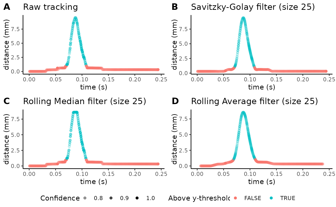

Notice how the transparency of each data point reflects the tracking confidence, as a qualitative way of assessing outliers. We’ll take apart the different settings for the plot_filter_graphs() function here, and then describe how we can optimize these settings to design an optimal filter for our data.

1. the csv_or_path variable refers to the path to the CSV you wish to track. Here, we’re looking at a trajectory for a manual stimulation in our sample dataset.
2. the p_cutoff variable refers to the confidence level at which you want to replace the data with interpolation. In other words, you might want to replace outlier points that were mistracked with interpolation between more confident points. Setting a p_cutoff of 0.1 replaces all the points that the model was <10% confident about with interpolation.
3. The reference_distance variable refers to the real-world distance between your two reference points. Our points in this example CSV were the top and bottom of a chamber (which we measured to be 40mm), so this value is set to 40. This distance will be used to adaptively calculate a scale factor for each video and scale your data appropriately, regardless of whether the camera you used was at different distances in different videos.
4. The manual_scale_factor variable can be used if you don’t wish to use reference objects to adaptively calculate scale factors. This is usually the case when you are certain your camera is always at the same distance away from your target, so you can enter a millimeter/pixel scale factor to be used for every single one of your videos. Keep in mind that setting a manual_scale_factor will override the reference_distance and adaptive calculations — the code will use your manual_scale_factor to scale all of your videos to scale them to millimeters.
5. The fps variable can be used to set the number of frames per second in your video to set a timescale for behavior. Here, we use 2000 fps. 6-8) The savgol_window_length, median_window_length, and average_window_length variables define the degree of smoothing (using either a Savitzky-Golay filter, a rolling median filter, or a rolling average filter) you wish to apply to the trajectory data. As a default, these values are set to 25, but you can increase or decrease the window of data-points each filter will use to apply smoothing. Generally, a higher window length results in increased smoothing, but be sure that by applying too high a level of smoothing, you are not suppressing any subtle behaviors. 9-10) For body_part, indicate whether you wish to show trajectories for the “toe,” the “center,” or the “heel.” For axis, indicate whether you wish to show trajectories for the given body part using the “x” axis or the “y” axis.

Next, we’ll look at how we can alter these parameters to optimize the levels of smoothing. The following code chunk plots trajectories from a mouse in the ARM group:

plot_filter_graphs(csv_or_path = lp_arm_stim,
                   p_cutoff = 0,
                   reference_distance = 40,
                   manual_scale_factor = NA,
                   fps = 2000,
                   savgol_window_length = 11,
                   median_window_length = 11,
                   average_window_length = 11,
                   fixed_baseline = 1,
                   y_threshold = 0.1,
                   body_part = "center",
                   axis = "y")
#> Warning: Removed 10 rows containing missing values or values outside the scale range
#> (`geom_point()`).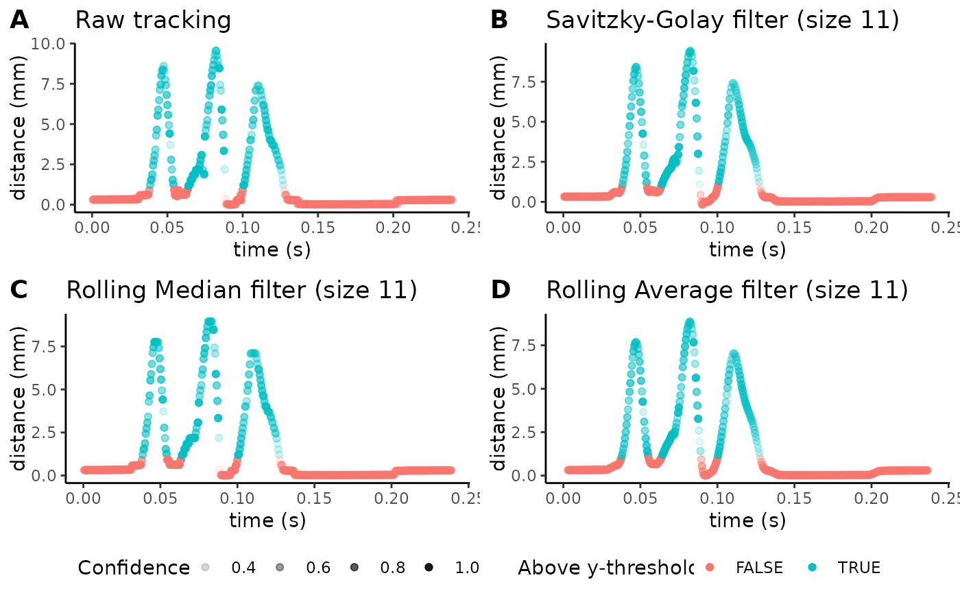

With more complicated trajectories (as the one we’re seeing above for the example ARM CSV), certain smoothing filters tend to work better than others. We’ve found that the rolling average filter (figure D above) tends to be the most robust. In this subplot, we see a very smooth trajectory (using filter windows of 11), but notice how it slightly reduces the maximum peak of the filter. Setting a higher filter window will dampen these peaks even further, so using this function is a helpful pre-processing step to optimize smoothing for a given video.

Finally, we’ll also increase the p-cutoff from 0 to 80% to see how data changes:

plot_filter_graphs(csv_or_path = lp_arm_stim,
                   p_cutoff = 0.80,
                   reference_distance = 40,
                   manual_scale_factor = NA,
                   fps = 2000,
                   savgol_window_length = 11,
                   median_window_length = 11,
                   average_window_length = 11,
                   fixed_baseline = 1,
                   y_threshold = 0.1,
                   body_part = "center",
                   axis = "y")
#> Warning: Removed 10 rows containing missing values or values outside the scale range
#> (`geom_point()`).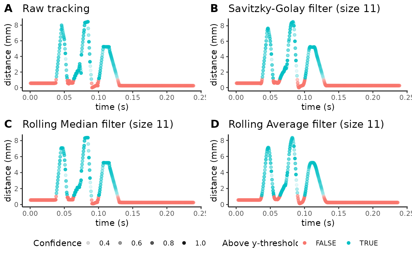

You will generally want to pick a p-cutoff based off of the confidence of your model’s tracking. Here, we’ve picked a p-cutoff of 0.8 (i.e. every point for which the model is 80% confident or less will be replaced with interpolation). You’ll be able to qualitatively visualize how tracked points with a confidence less than the p-cutoff threshold were instead interpolated between points that were above the threshold. As shown above, you can use this function to determine a balance between smoothing levels, the filter chosen for smoothing, and the p-cutoff to produce clean trajectories without suppressing subtle behaviors.

Running PAWS diagnostics

PAWS runs analysis primarily on a univariate projection — a combination of the x and y components, weighted based off of how much movement there is in a particular axis. It’s important to not only graph the raw trajectories of a paw over time in each axis, but also to graph the univariate projection and other diagnostic plots built into paws when troubleshooting or optimizing your workflow. To produce these plots using the settings from the most recent smoothing settings, you can run the following function:

plot_univariate_projection(csv_or_path = lp_arm_stim,
                   p_cutoff = 0.8,
                   reference_distance = 40,
                   manual_scale_factor = NA,
                   filter = "average",
                   fps = 2000,
                   average_window_length = 11,
                   fixed_baseline = 1,
                   y_threshold = 0.1,
                   body_part = "center")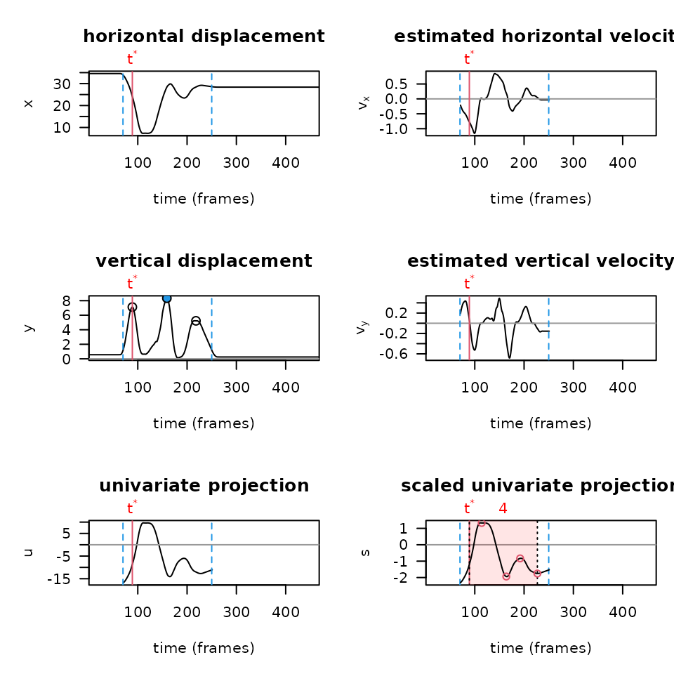

You’ll notice how the plots above are much smoother than if we run diagnostics on the same video, without smoothing the data first (shown below):

plot_univariate_projection(csv_or_path = lp_arm_stim,
                   p_cutoff = 0,
                   reference_distance = 40,
                   manual_scale_factor = NA,
                   filter = "none",
                   fps = 2000,
                   body_part = "center",
                   fixed_baseline = 1,
                   y_threshold = 0.1,
                   shake_threshold = 0.35)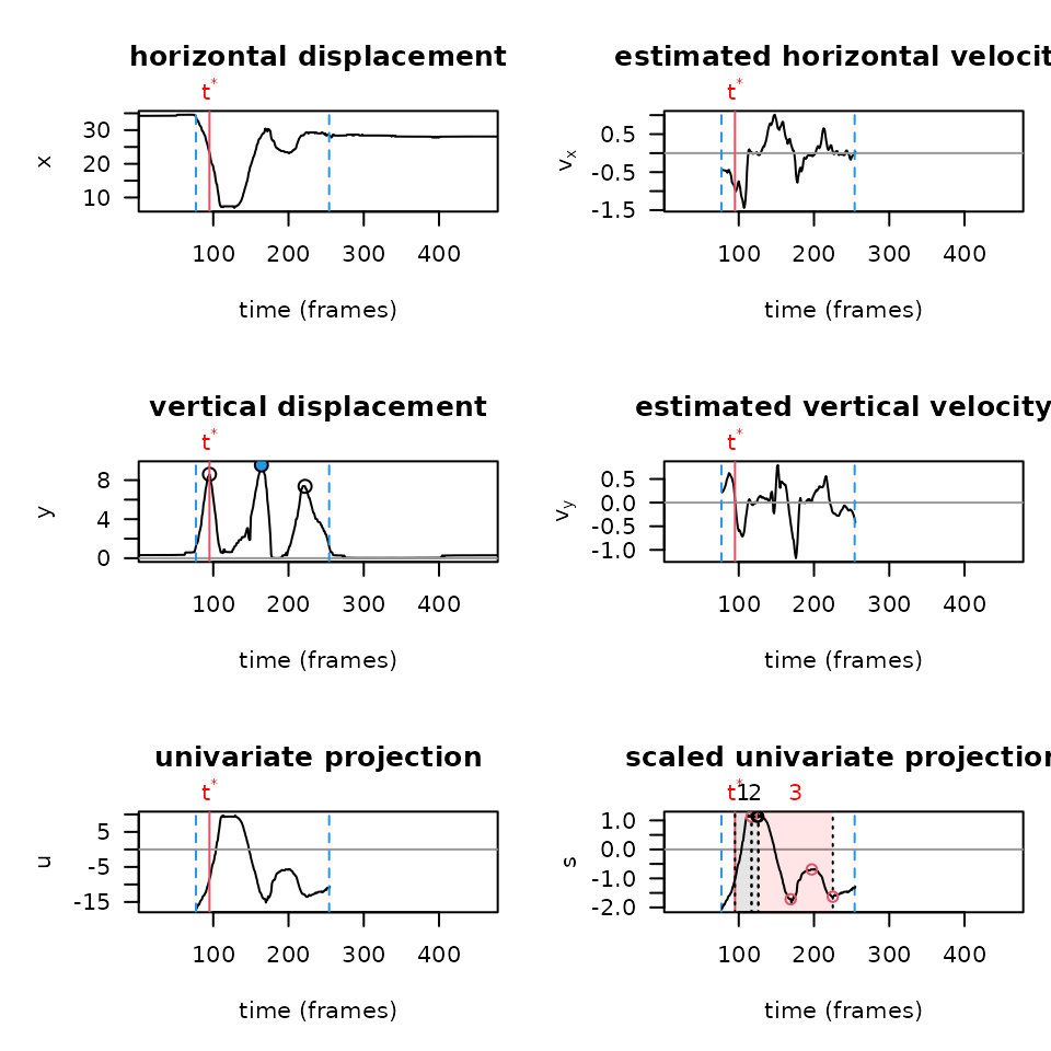

Above, you can also alter the shake_threshold parameter to make the PAWS algorithm more or less sensitive to detecting shaking behaviors (for instance, try changing 0.35 to 0.10).

Finally, one of the most important thresholds to set is the window_threshold, which specifies how sensitive PAWS will be in examining paw trajectories for a withdrawal behavior. Setting a lower threshold will result in higher sensitivity, while a higher threshold will result in lower sensitivity for paw withdrawal. If you have videos that aren’t being scored because the paw activity window was not found (especially common with innocuous stimuli), try setting a lower threshold.

Before running analysis on our entire dataset, we can prospectively see what the PAWS output for this video would look like by running the function mini_paws() on the toe, center, and heel body parts for our CSV:

toe <- mini_paws(
  csv_or_path = lp_arm_stim, p_cutoff = 0,
  reference_distance = 40, manual_scale_factor = NA,
  filter = "average", average_window_length = 11,
  fixed_baseline = 1,
  y_threshold = 0.1,
  fps = 2000, body_part = "toe"
)

center <- mini_paws(
  csv_or_path = lp_arm_stim, p_cutoff = 0,
  reference_distance = 40, manual_scale_factor = NA,
  filter = "average", average_window_length = 11,
  fixed_baseline = 1,
  y_threshold = 0.1,
  fps = 2000, body_part = "center"
)

heel <- mini_paws(
  csv_or_path = lp_arm_stim, p_cutoff = 0,
  reference_distance = 40, manual_scale_factor = NA,
  filter = "average", average_window_length = 11,
  fixed_baseline = 1,
  y_threshold = 0.1,
  fps = 2000, body_part = "heel"
)

lp_arm_manual <- rbind(toe, center, heel)
row.names(lp_arm_manual) <- c("toe", "center", "heel")

lp_arm_manual
#>        pre.pain_score post.pain_score pre.max_height pre.max_x_velocity
#> toe        -0.3116669      0.32753717       7.760343           1489.410
#> center     -0.4265664     -0.02546354       6.696816           1675.167
#> heel       -0.6157240      3.71363989       5.380741           1477.692
#>        pre.max_y_velocity pre.distance_traveled post.max_height
#> toe             1131.6070              12.20117       10.278125
#> center          1033.9974              12.06299        7.873508
#> heel             708.4806              10.23666       22.810259
#>        post.max_x_velocity post.max_y_velocity post.distance_traveled
#> toe               2483.291            1900.523               77.61317
#> center            2235.985            1606.068               70.06825
#> heel              1648.575            9296.099               98.83826
#>        post.number_of_shakes post.shaking_duration post.guarding_duration
#> toe                        4                0.0540                 0.0295
#> center                     4                0.0535                 0.0270
#> heel                       4                0.0245                 0.1650

Running PAWS

Finally, if we are happy with the degree of smoothing and diagnostic plots, we’re ready to run PAWS on a full set of CSVs. The paws_analysis() function uses many of the same parameters as were mentioned earlier, so we will show an example of how to run this using our sample dataset:

[note: the following code will throw a saving error because of how the R Markdown notebook is configured, but, if you are running this function in an RStudio environment, you can set a custom saveDirectory in the function to run it!]

paws_analysis(csvDirectory = "demo/sample_data",
              saveDirectory = "enter_save_path_here",
              p_cutoff = 0.8, manual_scale_factor = NA,
              filter_chosen = "average", filter_length = 11,
              reference_distance = 40, stims = "lp",
              body_parts = c("toe", "center", "heel"),
              reference_points = c("objecta", "objectb"), 
              groups = c("arm", "manual"), fps = 2000,
              shake_threshold = 0.35,
              fixed_baseline = 1, y_threshold = 0.1,
              withdrawal_latency_threshold = 4,
              expanded_analysis = TRUE)

You’ll notice two additional parameters at the bottom of this function: withdrawal_latency_threshold and expanded_analysis. Setting expanded_analysis to TRUE enable two additional variables to be exported: t* (t-star), the time-point at which the reflexive response turns into an affective response, and withdrawal latency, or the time-point after paw stimulation at which the paw is physically withdrawn. However, this expanded analysis can only be done under the assumption that the stimulus is applied at the very beginning of the video. If you are working with an experimental setup where you automatically begin recording videos when you apply a given stimulus (or you crop videos post-hoc so they are aligned in this manner), you can set expanded analysis to TRUE and include withdrawal latency in your analysis. Otherwise, the default for this setting is FALSE.

The second value, withdrawal_latency_threshold, determines how permissive the algorithm that calculates withdrawal latency will be. Higher values will be more accommodating (which you are encouraged to use if you have poor tracking, or use little smoothing), while lower values will be more stringent and require very little movement to trap velocity. Withdrawal latency is calculated by finding t-star, and then finding the closest time-point before t-star at which the velocity is zero (or near zero, with more accomodating thresholds).

You can also accomplish all of the previous steps and analysis using an interactive dashboard by running the following code:

paws_dashboard()